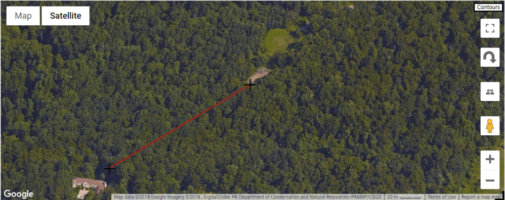
Path of 500 foot Beverage On Ground. Feedpoint is at upper right.
In the early part of 2018 I installed a 500 foot long Beverage antenna on the ground (BOG), and I have been pleased with its performance. With this antenna, I have been able to receive WSPR spots from Europe, Hawaii, Australia, and throughout the Continental USA and the Caribbean.
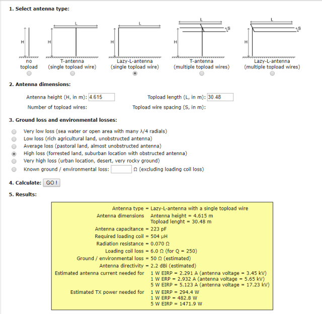
During the late Spring of 2018, I installed an Inverted L for use as a transmit antenna. Its vertical element is roughly 53 feet tall and the horizontal tophat extends for 210 feet.
The BOG runs along an axis of 230-250 degrees from its feedpoint to its termination. The Inverted-L runs along an axis of 12-25 degrees from its feedpoint.
I was curious how reception from the Inverted-L would compare with that of the BOG, so on the night of October 17, 2018 I set up two identical receive stations, with one station being fed by the BOG and the other being fed by the Inverted-L, and then I monitored both WSPR and JT9 on both stations from 0000 to 1200 UTC on October 18, 2018 and compared the results using the WSPRNet reports for each station (one station used the callsign W3SZ and the other station used the callsign W3SZ/IL).
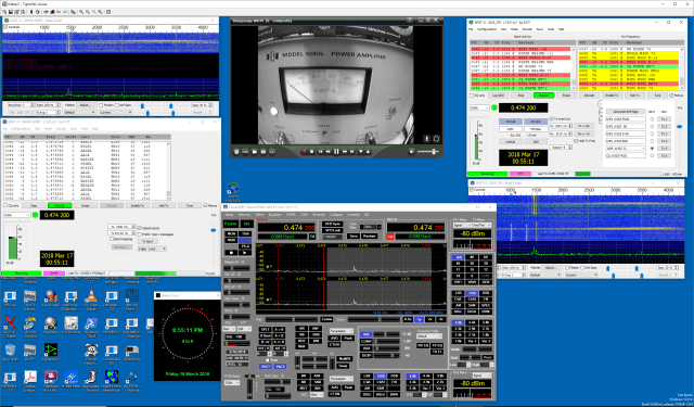
I used identical openHPSDR Hermes transceivers for this test. Each Hermes was running OpenHPSDR-PowerSDR mRx PS v 3.4.9 with two instances of WSJTX 1.9, one instance of WSJTX on each Hermes receiving WSPR transmissions and the other instance on each radio receiving JT9 transmissions.
I presented the results of that overnight comparison of these two antennas in mid October of last year. That comparison is here.
Those results were a bit surprising to me, which may just reflect my inexperience. The BOG DID do better than the Inverted-L, as I expected, but the performance difference between the BOG and the Inverted-L, while highly statistically significant, was not as large as I would have expected. Those results were performed before the 630M band had really “opened” for the year, and so I wanted to run another overnight test now that the band is open. This test was performed overnight on Janary 11 – January 12, 2019 which was a better-than-average night here at W3SZ, as you can see from my report which was included in John Landridge KB5NJD’s 630M Daily Report for today, here.
On WSPR on this January night, the BOG spotted a total of 1041 receptions. The Inverted-L spotted a total of 1046 receptions during the same time frame. The Inverted-L had more receptions because it copied my WSPR transmissions whereas the BOG did not. There were 948 simultaneous receptions by the two stations that allowed for direct comparison of simultaneously received signal strengths for the two antennas. Receptions were obtained of a total of 31 unique callsigns. 14MDA, DL6TY, EI0CF, F1AFJ, KR6LA, LA3EQ, PA0A, and PA3ABK were received only by the BOG. W3SZ (as noted above) was received only by the Inverted-L. The remaining 23 unique callsigns were detected by both antennas. There were 93 Receptions that were made by the BOG that were not detected by the Inverted-L, and 48 receptions (other than W3SZ) that were made by the inverted-L but not by the BOG.
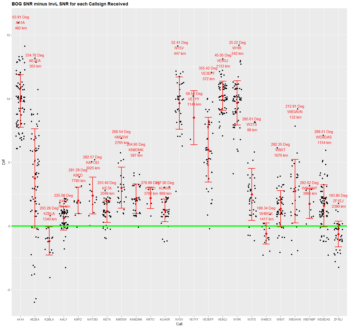
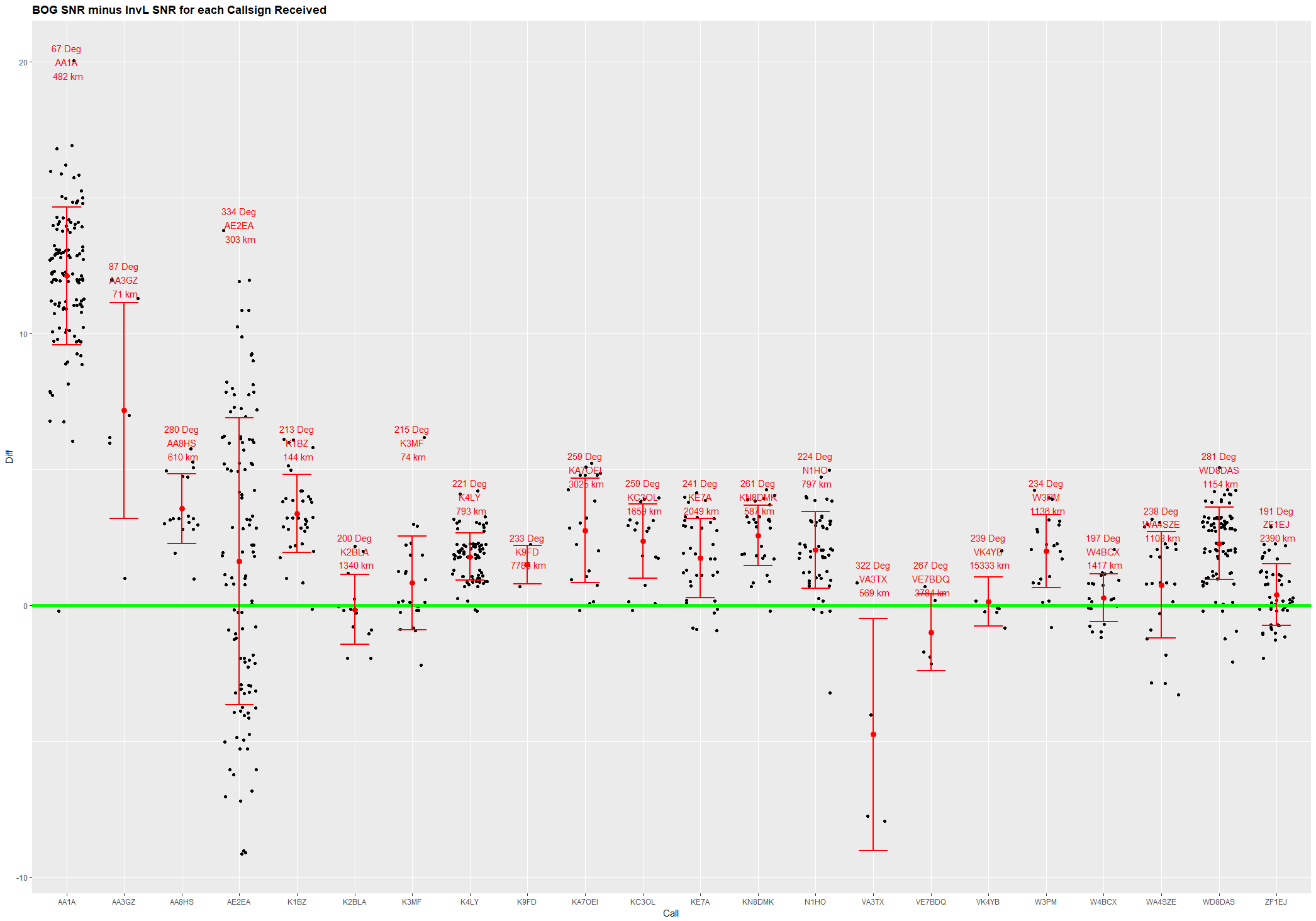
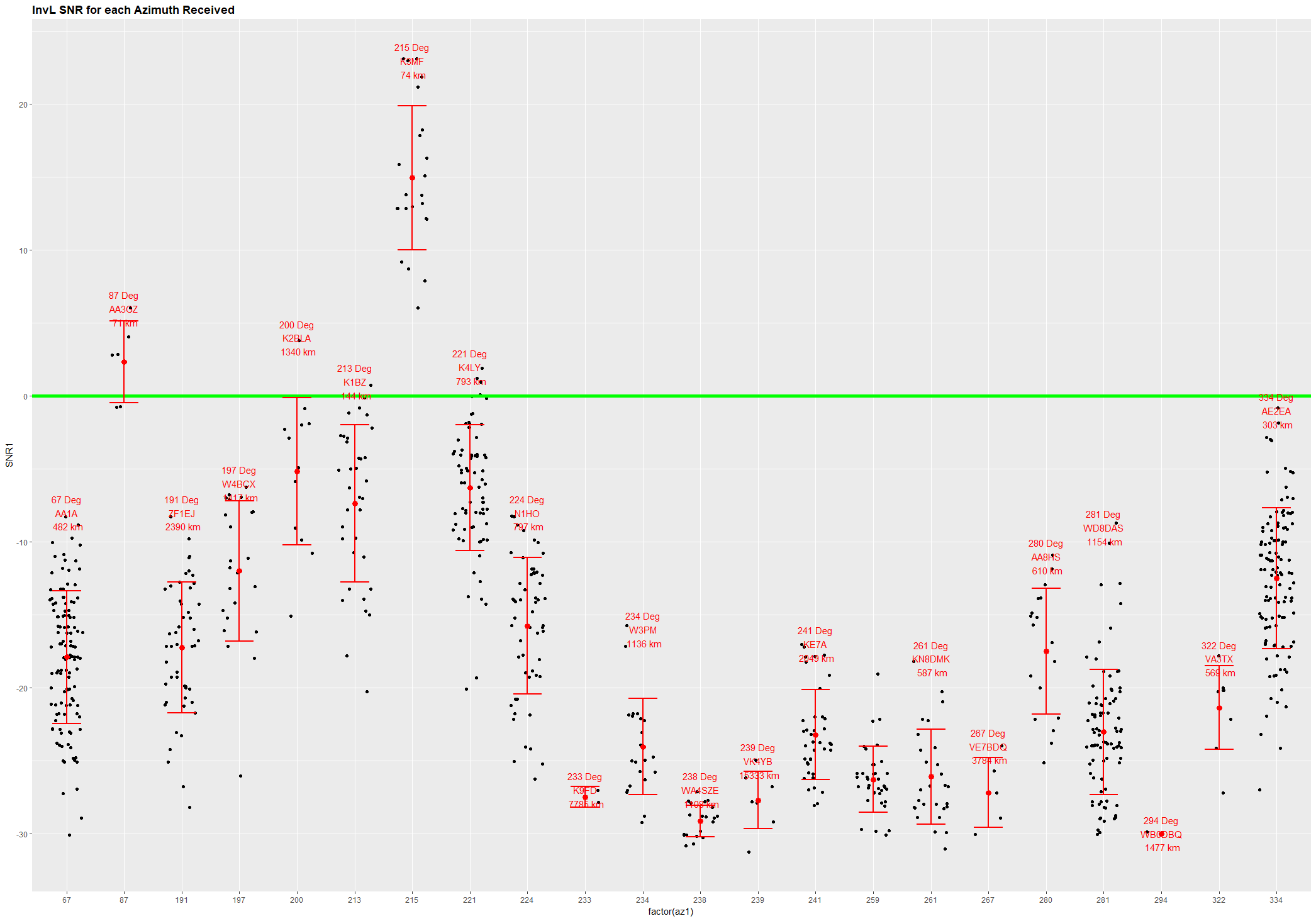
The graphs below will show signal strength (or difference in signal strength) in WSJT units (dB) on the Y axis, and either callsign or azimuth on the X axis. For each X value all data points for that X value will be shown, along with the mean and standard deviation error bars for those values. In addition, to make interpretation easier, the Azimuth, Callsign, and Distance to the received station from FN20ag (W3SZ location) will be shown in red near the upper error bar. Where that text data is not given on the graphs of signal strength vs azimuth, the omission is because two or more stations shared a single azimuth value. A horizontal green line will mark the 0 dB signal level on each graph.
The first graph below compares the signal strengths of simultaneously received signals on the BOG and the Inverted-L by displaying the value (BOG SNR minus Inverted-L SNR) vs Callsign. A positive value (above the green line) indicates that the BOG heard better than the Inverted-L, and a negative value (below the green line) indicates that the Inverted-L heard better than the BOG. As indicated above, the mean Y value for each X value is shown in red, as are the error bars above and below the mean value. 20 of the 23 stations received by both antennas were on average heard better on the BOG than on the Inverted-L.
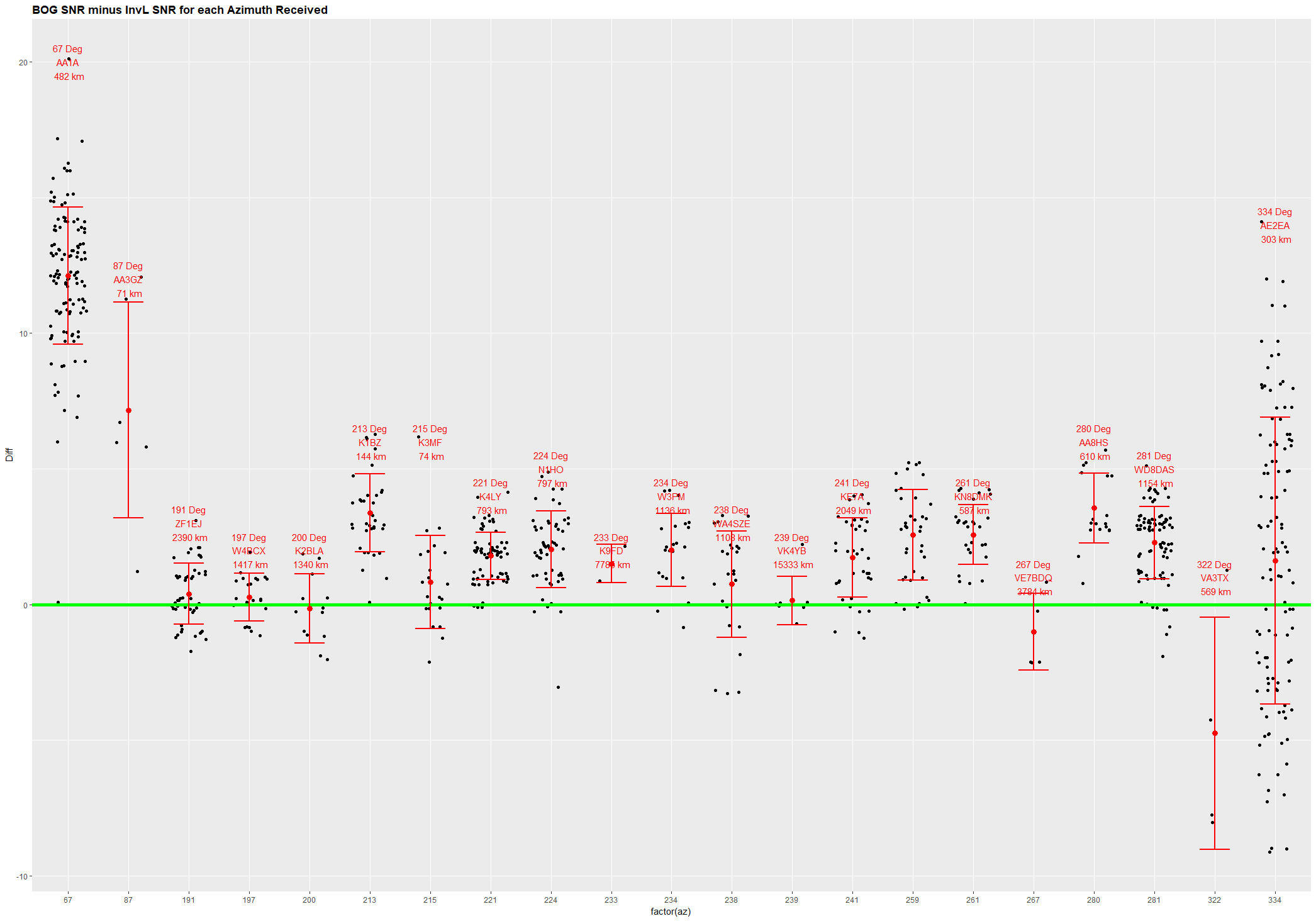
The graph below shows the same parameter displayed for the Y values, (BOG SNR minus Inverted-L SNR), but the X axis parameter is now azimuth of the received station from W3SZ. You can see that the greatest advantage of the BOG was between 334 and 64 degrees (and especially between 0 and 64 degrees), over a range of approximately 90 degrees, centered at approximately 20 degrees azimuth. The stations between 0-64 degrees had 8-10 dB better SNR on the BOG than on the Inverted L. The 3 stations between 194 and 204 degrees azimuth were the only stations that had worse SNR on the BOG than on the Inverted L. This difference was slight, only 1-1.5 dB.
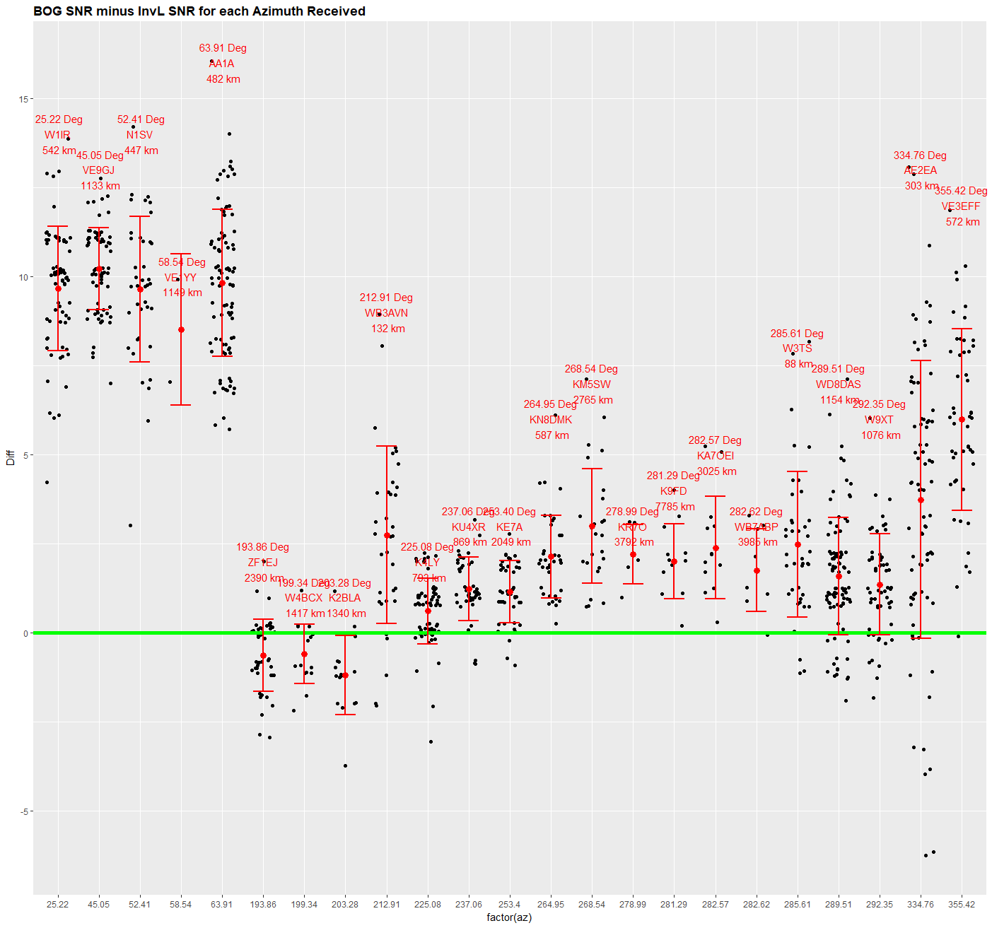
As you can see in the graph immediately above, 16 of the 23 stations had the error bars completely above the green 0 dB line. Only one station, K2BLA, had the error bars completely below the green 0 dB line. A t test of all of the simultaneously received BOG and Inverted-L signal strength results gave a p value of 2 x 10-16 for the comparison. In general, a p value of less than 10-2 is considered to indicate a significant difference, so this results indicates a highly significant difference between the received signal strengths of the BOG and Inverted-L antennas, in favor of the BOG. Although the mean difference between the two antennas was 4.2 dB SNR, there was great directional variation as noted, from 10 dB advantage for the BOG over 0-64 degrees azimuth to 3-6 dB advantage for the BOG for 334-360 degrees, to 1-3 dB advantage for the BOG for 213-293 degrees, to 1-1.5 dB deficit for the BOG from 194-204 degrees.
Of course, these graphs don’t show the azimuths of the stations that only the BOG received, namely DL6TY, EI0CF, F1AFJ, KR6LA, LA3EQ, PA0A, and PA3ABK. These stations have azimuths (listed in ascending order) of 41, 44, 47, 47, 49, 56, and 286 degrees. This provides further evidence of the substantial superiority of the BOG in the azimuth range of 0-64 degrees.
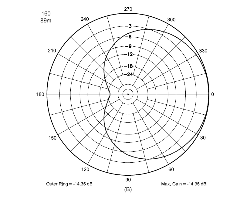
Interestingly, the BOG does not have an obvious peak in its performance relative to the Inverted-L in its “preferred” direction of 230-250 degrees pointing along its axis and directed away from its feedpoint. Of course, a 500 ft BOG would not be expected to have much directivity at 630M, for its wavelength assuming a velocity factor of 55% would be only (500/0.55 * 12/39.37)/630 = 277/630 = 0.44 wavelengths. So it would be even less directional than the elevated 89m-long 160M (0.56 wavelength) Beverage in this illustration taken from ON4UN’s text where the -3 dB points are at approximately +/- 70 degrees:
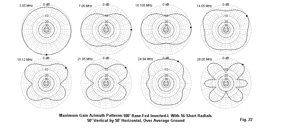
And my Inverted-L, if I am interpreting L.B. Cebik’s work correctly, would have minimal if any directivity on 630M; see the plot below for a 50 x 50 Inverted-L on 3.55 MHz. With my Inverted-L dimensions, at 630M my Inverted-L would be expected to be even less directional than the plot for 3.55 MHz in the illustration below, and the azimuth plot of the 3.55 MHz antenna is nearly a perfect circle:
What is really surprising to me is that azimuth range where the biggest advantage for the BOG is seen is at azimuths centered around 20 degrees, which is close to the “180 degree” expected null of the BOG, which would be expected to be between 50 and 70 degrees. And we can’t explain this anomaly by invoking directivity of the Inverted-L, because that should have almost no directivity.
I guess other explanations must be in play here; perhaps including the signals angles of arrival at each antenna, distortions of one or both antenna’s expected patterns by local terrain and adjacent structures, the unavoidably asymmetric ground system of the Inverted-L (due to adjacent buildings), and other factors.
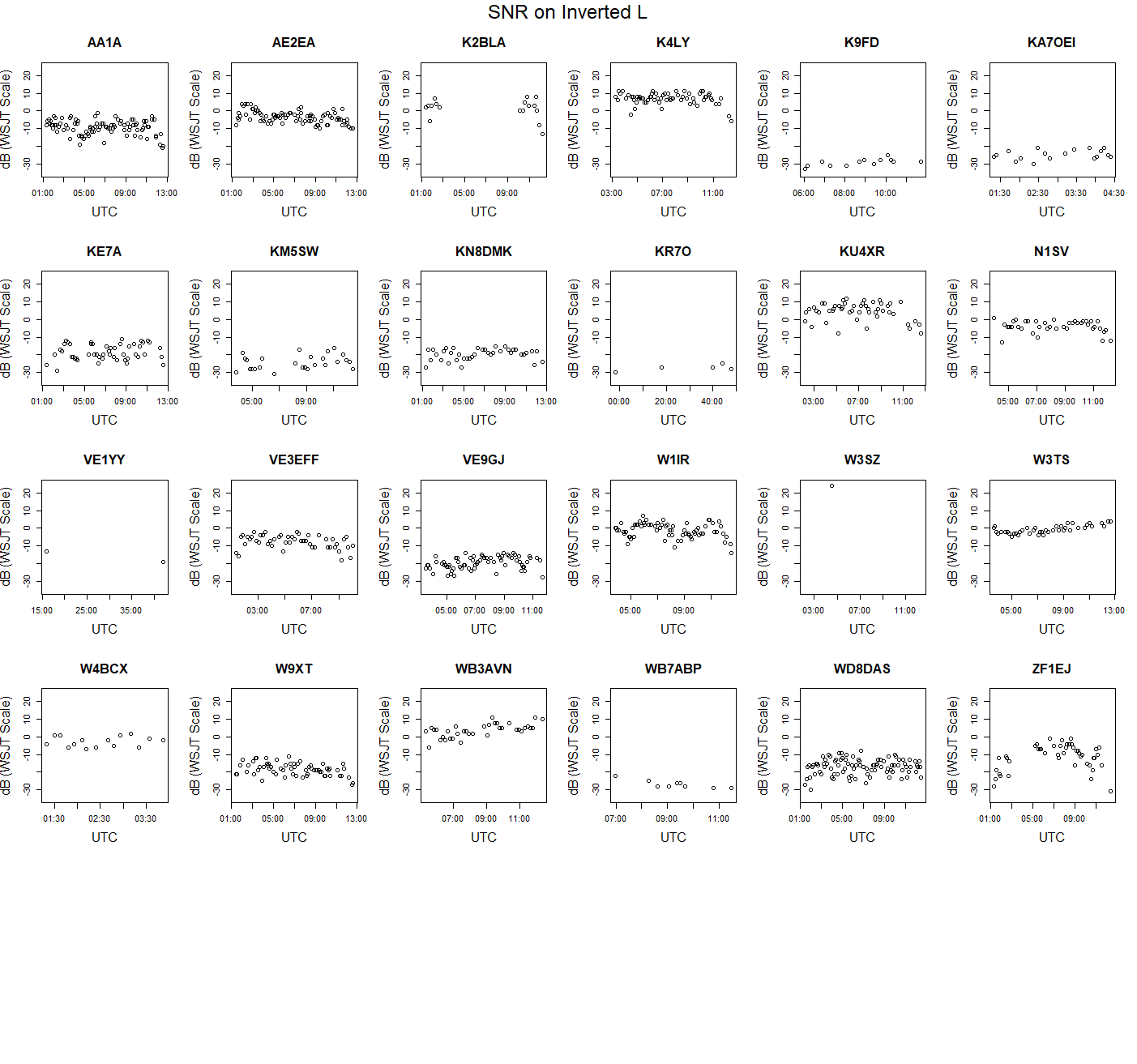
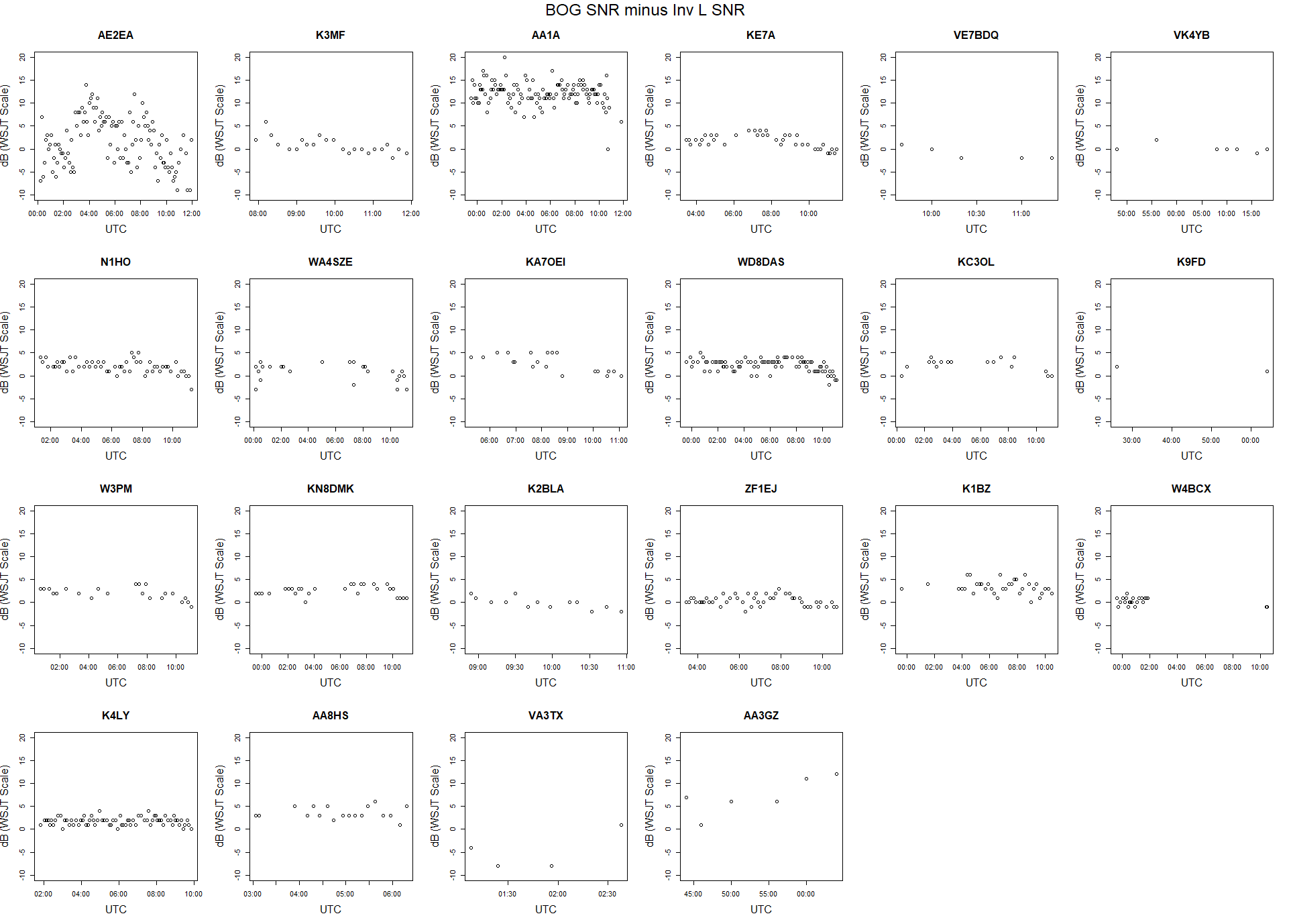
To sort this out, I thought that it might be helpful to look at the difference in signal strengths between the two antennas for each callsign/azimuth received as a function of time, so I produced the graph below. It shows a small graph of (BOG SNR minus Inverted-L SNR) vs time for each simultaneous reception for each callsign received. In other words, it plots the difference in dB of the SNR for signals simultaneously received by both antennas vs time for each individual station received. I set this up so that the X axis will autoscale for each individual graph to give the best display of datapoints for that particular station. As a result, the X axes differ from graph to graph, so stay alert as you peruse this image. If the image is too small for you to view it comfortably, you may find it helpful to right-click on the image and then open it in a separate tab so that you can enlarge it to better see the details. A few of the graphs (e.g. KR7O, VE1YY) where the station was only received over a very short interval show minutes instead of hours on the X axis:
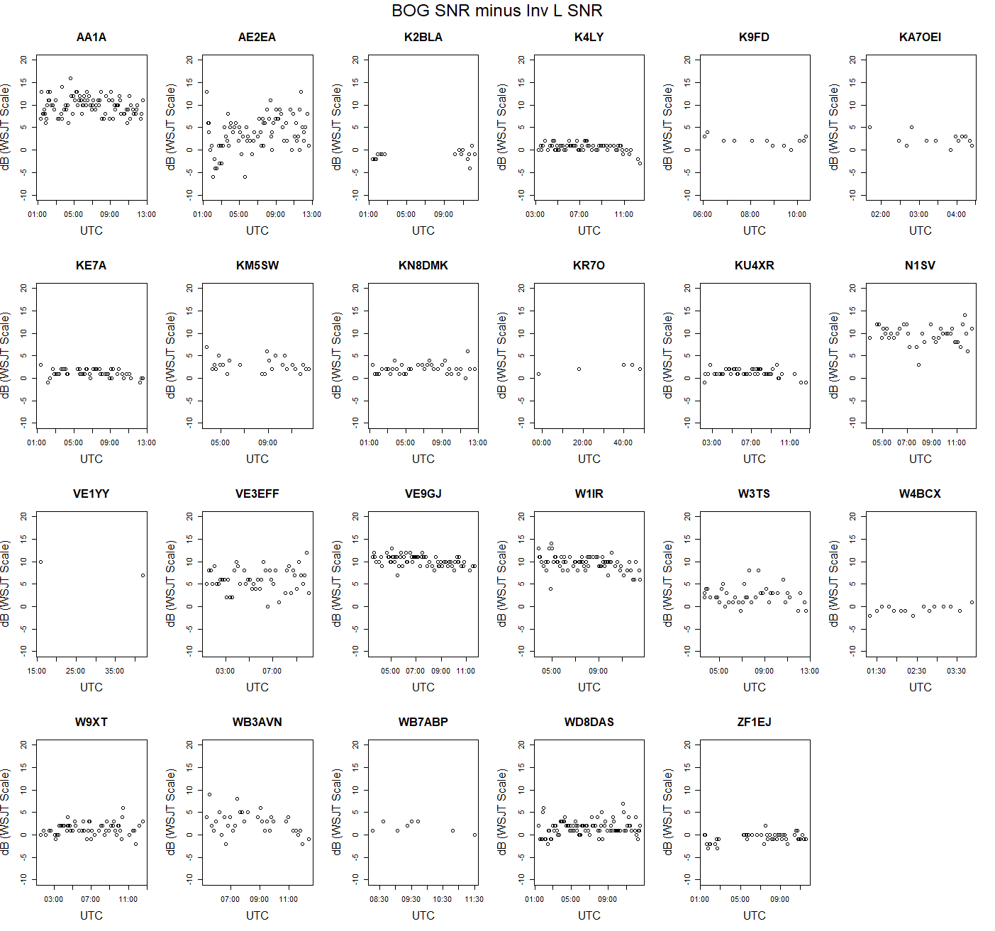
Unfortunately, this analysis provided me with no additional insights regarding the mechanisms causing the substantial relative performance differences between the two antennas at different receive azimuths. There was a suggestion that the difference between the two antennas tended to diminish after approximately 1000 UTC in some cases, as the band “closed” for the day.
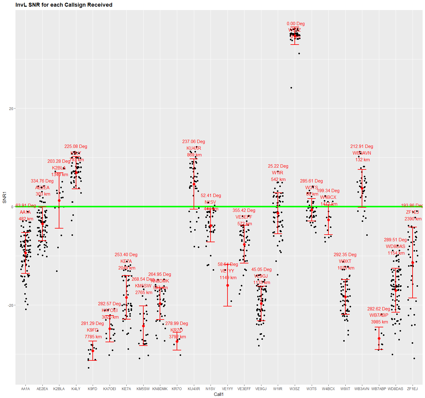
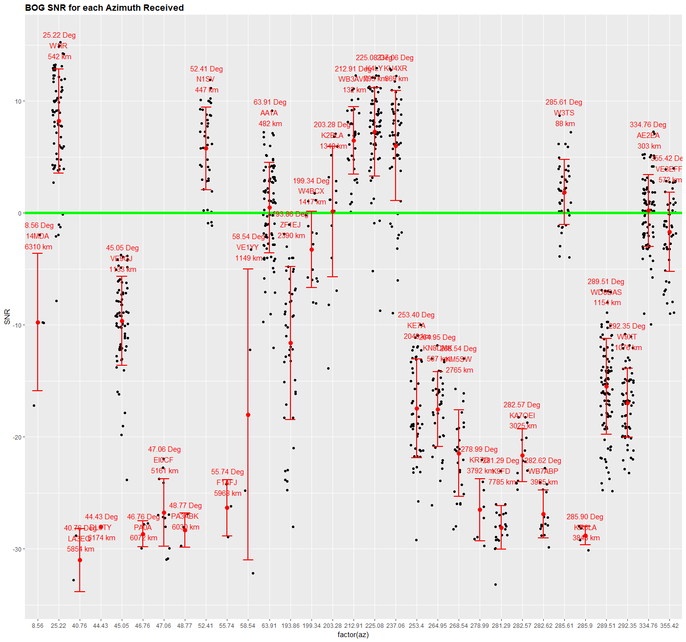
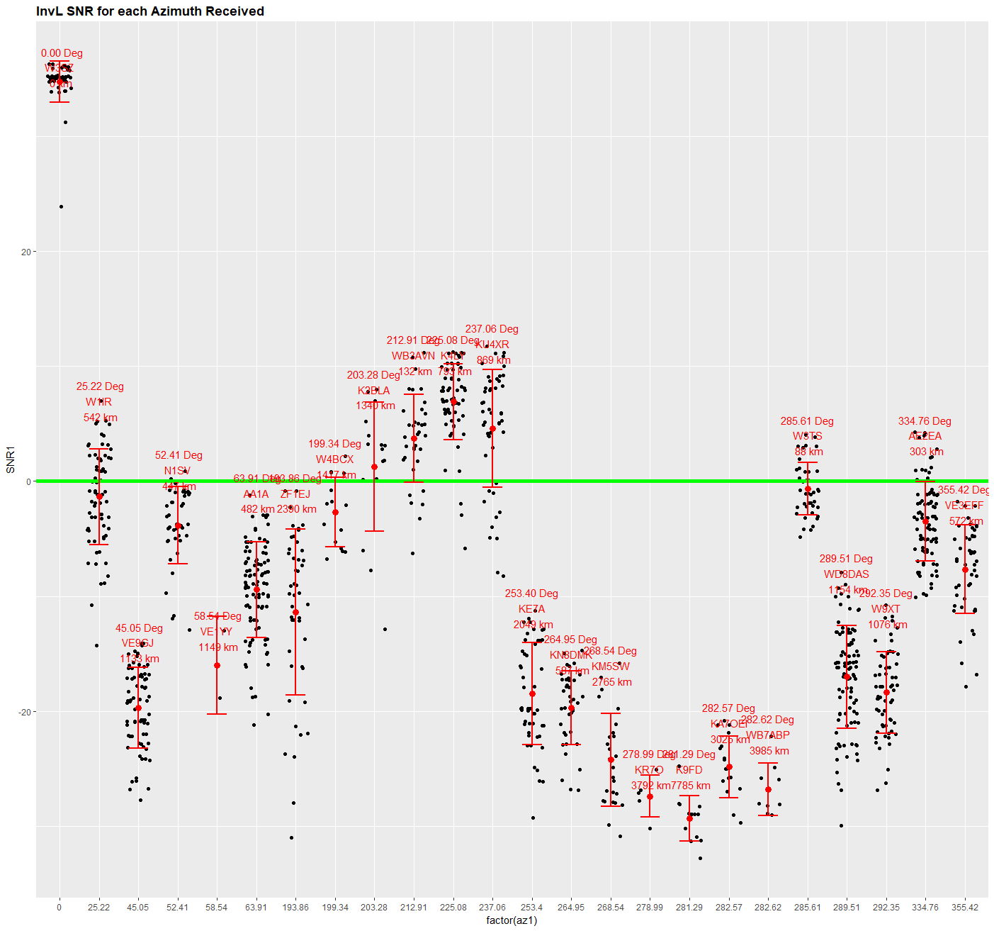
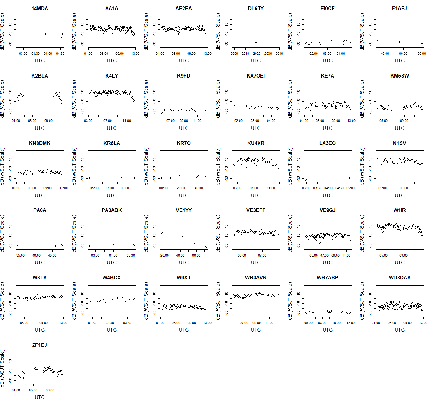
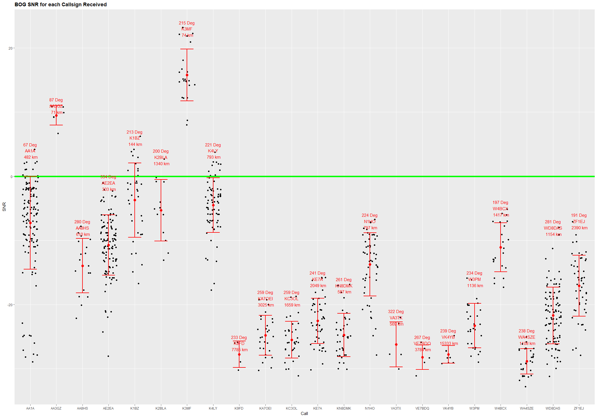
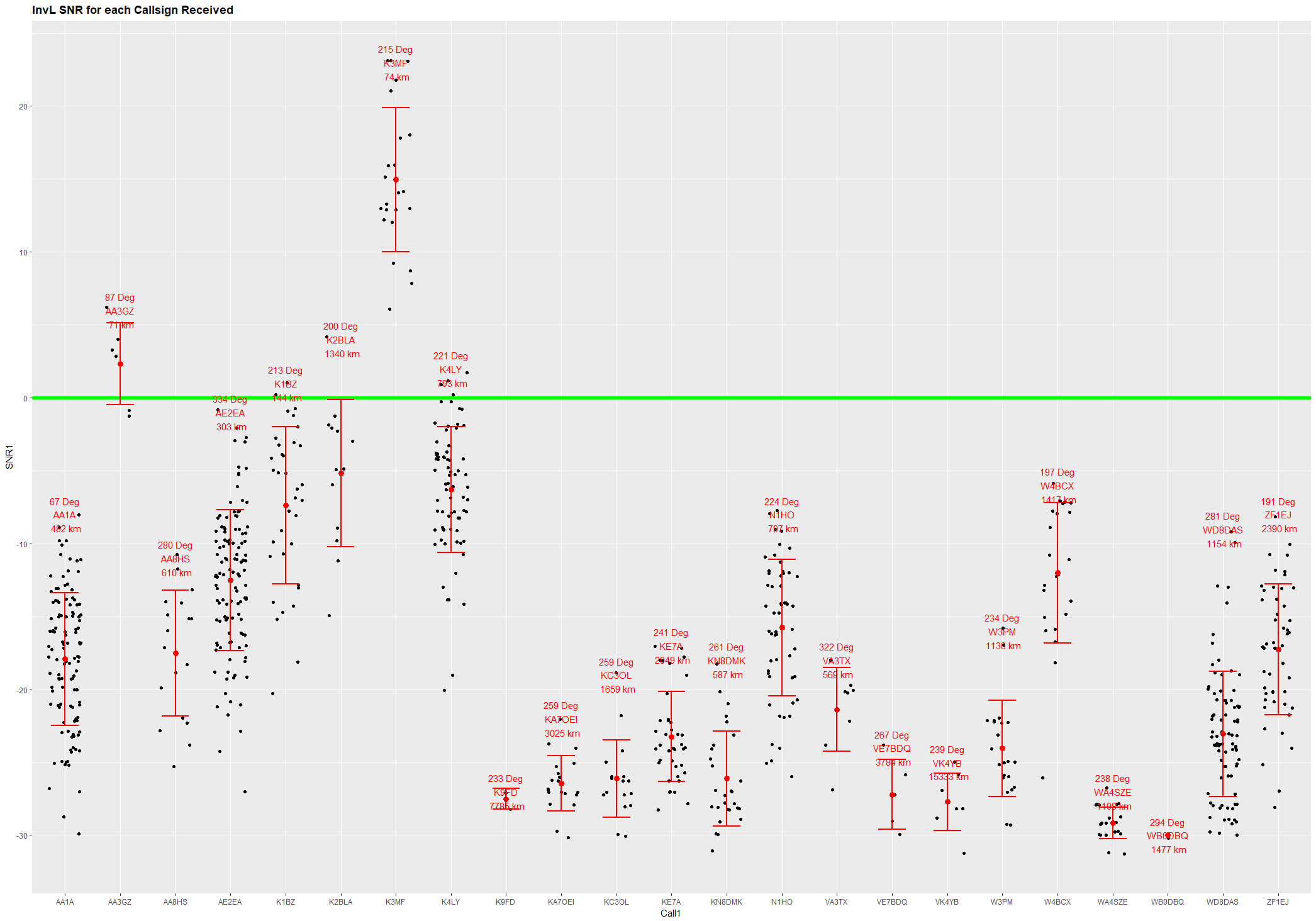
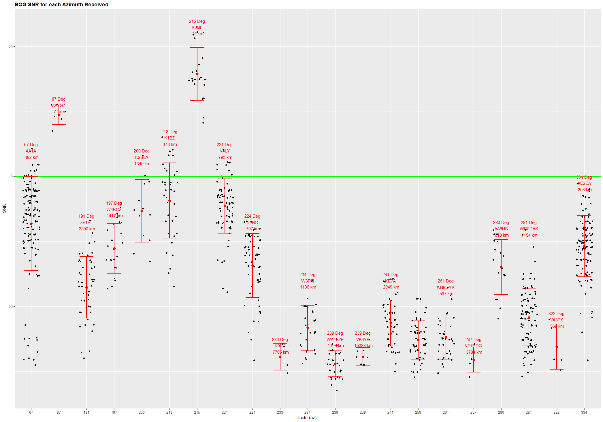
Below are, without comment, some graphs of the raw data for each antenna with means and error bars shown, with x axis factors as above being either Callsign or Azimuth from W3SZ.

The graph below lacks a title. It shows SNR vs Time for the BOG.
Compared with the prior results that were obtained in October, 2018, the differences between the two antennas are much more apparent on the current study, likely because the “openness” of the band provided a much greater variety of signals for the current analysis than was present in October.
73,
Roger Rehr
W3SZ


 Next pull the red bandpass filter line in the bottom right corner to the right until it disappears off the screen. You will see the frequency of the bandpass edge increase as you do this. I pull it all the way to 192000, which is well outside the HDSDR window.