Just Testing

NJD Technologies’ Blog pages by KB5NJD, John Langridge, are one of the best sources of information I’ve found for 630m (and 2200m).

W5EST put some of the information in these blog entries into book form.  The book has 22 chapters.

I could not find a set of easy links to these, so I have made a set of links to the chapters here.

Chapter-1_Distinguishing630.pdf

Chapter-2_RX-Antennas.pdf

Chapter-3_RXs-Decoders-630.pdf

Chapter-4_Local-Noise-630.pdf

Chapter-5_Operating-Modes.pdf

Chapter-6_Storms-Band-Noise.pdf

Chapter-7_Common-Darkness.pdf

Chapter-8_Spatial-Diversity-Screen-Sharing.pdf

Chapter-9_630mPaths_Short-Medium.pdf

Chapter-10_TX-Antennas-Hats-Grounds.pdf

Chapter-11_Antenna-System-Concepts.pdf

Chapter-12_ATUs-Matching.pdf

Chapter-13_TXs-PAs.pdf

Chapter-14_TR-Station-Controls.pdf

Chapter-15_Daily-Regimes-Annual-Seasons.pdf

Chapter-16_Etiquette-Band-Planning.pdf

Chapter-17_Propagation-on-Long-Paths.pdf

Chapter-18_QSB.pdf

Chapter-19_630mDaytime-Solar-Eclipsesa.pdf

Chapter-20_Propagation-Mysteries.pdf

Chapter-21_Analyzing-Information.pdf

Chapter-22_630m-Future.pdf

Learn and Enjoy!

73,

Roger W3SZ

 

The graph above is a comparison of signal levels for 630m WSPR signals simultaneously received at my station between December 10 and December 12, 2017 on the 500 foot BOG “aimed” at 250 degrees azimuth and the 200 foot BOG aimed at 40 degrees.  You can see that nearly 10,000 signals were simultaneously received.

Each black data point represents (signal strength in WSJT dB units received on the 250 degree BOG minus signal strength in WSJT dB units received on the 40 degree BOG).  Mean and standard deviation for all data points for each callsign are shown in red.  The horizontal green line shows 0 dB, so points above this line had stronger signals on the 250 degree (500 foot) BOG, and points below this line had stronger signals on the 40 degree (200 foot) BOG.

You can see that the vast majority of the signals were received more strongly on the 250 degree, 500 foot BOG and that there does not appear to be a significant directionality to the difference between received signal strengths for the two antennas.

This is not surprising.  Although Beverage antennas are directional, their directionality depends on their wavelength, and significant directionality begins at approximately 0.25 wavelength.  As length increases, so does directionality.  At 630 meters (474 kHz), my 500 foot BOG has a length of 0.24 wavelength ignoring velocity factor.  If one assumes a velocity factor of 0.5, the 500-foot BOG would have length of 0.48 wavelengths.  But the 200 foot BOG would have length of less than 0.1 wavelength without considering the velocity factor, and even considering a velocity factor of 0.5, the length would be only 0.2 wavelengths.  So one would not expect to find significant directionality when comparing these two antennas.  Obviously, at 136 kHz the directionality of these antennas would be even less, as the wavelength at that frequency is approximately 2200 meters.

You can see that on average, the 500 foot BOG is on the order of 5 dB better than the 200 foot BOG. In a prior post I showed that this shorter 200 foot BOG was 5-15 dB better than my 40 foot inverted L antenna. And in a post prior to that one, I showed that the 40-foot inverted L was 5-10 dB better than the first inverted L that I had installed, which I ran between my two towers. So, starting with a relative reference signal level of 0 dB, I improved the relative signal to 5-10 dB with the second inverted L. The 200 foot BOG improved the relative signal to 10-25 dB. And going to the 500 foot BOG improved that to 15-30 dB. So a signal that with my first antenna would have been -30 dB would be -15 to 0 dB with the 500 foot BOG. Quite an improvement!!

What is happening on the graph above at 242.5 Degrees with the WA4SZE signal? Well, WA4SZE has a notoriously terrible signal and has WSPR signals on at least 4 separate frequencies, each with a different signal strength.  A gross test of your receiver’s capability is how many spurious WA4SZE signals you can receive at once on the 630 meter band.  I did not take the time to separate out the individual signals from WA4SZE for this analysis, and so sometimes the WA4SZE spurii with weaker signals on the 500 foot BOG were compared with the WA4SZE signals with greater signal strength, thus producing the strange graphic result above.  This graphic anomaly could be corrected by evaluating each frequency component of the terrible WA4SZE signal separately, but it is not worth taking the time to do that.  Who knows, maybe someday WA4SZE will even clean up his signal!

My BOGs are lying directly on the ground.  At one end there is a transformer to match the antenna impedance to the coaxial line, and at the other end each Beverage is grounded to a 4 foot ground rod through a 220 ohm resistor.  The transformers were taken from a 160 meter installation.

In addition to monitoring the WSPR signals as noted above, I also monitored JT9 traffic on 630m for two nights, using the 40 degree, 200 foot BOG.  With this I copied 23 separate stations transmitting JT9, and 707 JT9 signals.  Below is a set of graphs showing the signal strengths for each of the 23 JT9 stations copied vs time:

 

 

Many of these stations are also represented in the WSPR data given above and also given in prior blog posts.

I also compared the relative signal strengths when using these antennas on 136 kHz.  This dataset was also acquired over two nights from 12-10 through 12-12, but this dataset only has 947 datapoints divided among 3 stations, one of which is in Maryland and two of which are in Arizona.  You can see that the 250 degree, 500 foot BOG is about 5-6 dB better than the shorter antenna:

 

 

Below is an image of what happened when I connected a new “wall wart” to one of the SDRs so that I could independently power it up and down. The vertical lines on the waterfalls are birdies that are not caused by the wall wart. All of the diagonal lines represent spurious signals generated by the wall wart that gradually drift upwards in frequency. The device is a ZOZO Multivoltage switching AC power adapter called the “ZOZO 12W Multi Voltage Charger” that I purchased at Amazon. You might want to avoid it. Here is the image:

Buyer Beware!

Finally, below is an image showing my bandscope for 136 kHz receive on the 200 foot BOG on top, and for the 500 foot BOG on the bottom. Note the horizontal noise bands on the 200 foot BOG tracing. The 200 foot BOG roughly parallels (and in the horizontal dimension is within 5 feet of) the main underground 220 VAC service coming into my shack for roughly 2/3 of its (the BOG’s) length. The mains supply actually crosses under the BOG as the mains supply approaches the shack. In contrast, the 500 foot bog is at its closest 150 feet from the power line, and extends to 650 feet away from the power line. On the spectrum display, the noise that produces the horizontal bands on the waterfall is seen of course as the noise floor rising above the “quiet” baseline and then dropping back down to the baseline between noise events.

73,
Roger
W3SZ

Yesterday I installed my first BOG (Beverage On Ground) at Hilltop.  Russ, NN3Q, was kind enough to loan me two 200-foot BOGs with transformers that he had taken out of service on 160 meters.  So the BOGs are a bit short for 630m and 2200m, but i figured that I would give them a try.

The impedance of an above-ground Beverage is generally on the order of 400-450 ohms, but that of a BOG is lower, on the order of 200-250 ohms.  A beverage should be terminated with a total resistance to ground equal to its characteristic resistance.  So the sum of the ground rod resistance plus the terminating resistance for a BOG should be 200-250 ohms.  I used a 220 ohm resistor, which is likely too high, as ground rod resistance is likely on the order of 50-350 ohms, depending on soil conductivity, according to ON4UN’s Low-Band DXing.

I wanted to run the beverage along an azimuth of approximately 50 degrees, to cover Europe, and I ended up with a heading of about 45 degrees, I think, as you can see on the satellite map above.

Russ suggested that I first try the BOG without a preamp, but I wanted to have a preamp available if it was needed, so I hooked up a DX Engineering RPA-1 which has the feature that when it is powered down it is bypassed, making it easy to take it in and out of the circuit remotely. I had turned it on initially to make sure it would power up, and so it was turned on when I had my first look at how the BOG behaved. The table below shows what I saw in the first 5 minutes or so after activating the BOG:

Station /band kHz	Signal Level – BOG with Preamp On	Signal Level – BOG with Preamp Off	Signal Level: 40 foot wire
K3RWR 0.136	-27 dB	-9 dB	-15 dB
W3LPL 0.4742	-17 dB	-2 dB	-6 dB
AA1A 0.4742	-17 dB	-8 dB	-9 dB
WA3ETD 0.4742	nil	-15 dB	-18 dB

The numbers with the preamp on were surprising. I figured that they meant that either the preamp was being overloaded or the strong signal it was putting out was causing overload further down the receive chain and thus the worsened numbers, or something was wrong with the preamp. The preamp had been working fine previously, so my bet was that overload was the problem. I took the preamp out of the circuit and checked it, and it IS fine…slight increase in noise floor and 20 dB increase in signal strength at 0.474 MHz as viewed on my 141T when it is placed in the circuit and powered up.

But you can see from the table that WITHOUT the preamp, the BOG appeared to be 1-6 dB better than the 40 foot inverted L, depending on the azimuth.

I ran WSPR receivers overnight on both the BOG and the 40 foot inverted L, and I accumulated 745 simultaneously received datapoints. You can see them on the graph below:

The graph may be easier to see if you open it in a separate tab. It shows the signal difference between the Inverted L and the BOG with this difference expressed as inverted L signal strength in dB minus BOG signal strength in dB. The horizontal green line is the x axis. So points above the green line are those where the Inverted L was superior, and those below the green line are those where the BOG was superior.

You can see that most of the points are below the green line, indicating that most of the time the BOG was better. The two antennas were not statistically different at 63 degrees or 272 degrees. The Inverted L was better at 284 and 290 degrees. At all other azimuths the BOG was better by 5-15 dB ( 25, 32, 194, 200, 219, 225, 228, 261, and 357 degrees).

It is difficult to know what to make of the azimuth data given that we don’t know the pattern of my inverted L. The axis of the horizontal element of the inverted L is 123 degrees, so broadside would be 33 and 213 degrees, so one might guess that those directions would be favored for the inverted L. But the length of the inverted L’s horizontal element is such a small fraction of a wavelength (18.8/630 = 0.029) that the inverted L likely has little if any directivity (see for example figure 18a and 18b of L. L. B. Cebik’s paper, “Straightening out the Inverted L”).

The axis of the BOG, as you can see in the image at the top of this page, is about 45 degrees. So the main lobes of the inverted L and the BOG would be expected to have similar azimuths (33/213 degrees for the inverted L and 45 degrees for the BOG) but this is not apparent in the data. There are likely several reasons for this. First, the take-off angles for the two antennas are likely different but complex functions of azimuth for the two antennas. Second, the pattern of the secondary lobes and nulls for the two antennas is likely very different.  Third, the 200-foot BOG is extremely short from the standpoint of its wavelength, and so like the Inverted L, it may actually have little or no directivity.

It would be advantageous to have a longer BOG, but in the direction of my first BOG I do not have enough room, if I start the BOG at my fenced-in compound. Also, from 50 degrees to 200 degrees azimuth I don’t have enough room for a BOG if I start it at the fenced-in compound. But from 200 degrees through 30 degrees I have room for beverages of 400-500 feet starting at the fenced-in compound; perhaps not ideal, but significantly better than at 50 degrees. If I run a Beverage from one end of the property to the other at 45 degrees or so, I can get about 800 feet of Beverage, although that would require a feedline length of 400 feet. If I run a Beverage from one end of the property diagonally at 250 degrees (good for Australia and New Zealand) I can get about 600 feet of Beverage.

So the question is, how long should a BOG be for 630m? Generally 1 wavelength is said to be the minimum “ideal” length for an above-ground Beverage. But BOGs can be shorter than this, because while the velocity factor for a Beverage in air is on the order of 95-98%, the velocity factor for a BOG is on the order of 50-60%. So BOGs can be (in terms of their physical length, ignoring the velocity factor) 0.5 to 0.6 wavelength long and have an electrical length of one wavelength. Thus, in the 630m band a BOG would ideally be 315-378 meters or 1033-1240 feet long. So even at the maximum length that I can accommodate my Beverages will be less than ideal. But I could get close, if I used the full extent of my property. The downside to that would be disruption of the Beverages by (illegal) hunters, trespassing hikers, and critters.  And my current BOG is less than 0.2 wavelength long, assuming a velocity factor of 50%.  So it is not surprising that I did not detect any directivity along the axis of the BOG.

I also evaluated this short 200-foot-long BOG on 135 kHz, but that is a subject for another day.

References: There is a good reference on Inverted L antennas here. I had previously referenced W8JI’s excellent receiving antenna notes as well as his section on Beverages. Here is another web page with some hints on BOGs, by K1FZ.

73,

Roger
W3SZ

I heard my first signals and got my first decodes last night on the 2200m / 0.136 MHz band!

My first decode, which came immediately on my tuning to this band, was from WH2XND in DM33, 3356 km away from my QTH, with a signal strength in WSJT units of -27 dB. WH2XND was copied for most sequences between my start time of 0456 and 1120 UTC, when I received the last decode from him for the night. His best signal strength here was -24.

Immediately thereafter, at 0458, I copied Rob, K3RWR at -15 dB, again in WSJT units. Rob was also copied essentially every sequence through the night, with my last decode of K3RWR at 1306. Rob is only 213 km away, and his strongest signal was -6 dB.

I also copied WH2XXP, who is close to WH2XND. They are both in DM33, near Phoenix, AZ. XXP was copied frequently, but less often than the other two stations mentioned, and only between 0608 and 1032. His strongest signal was -26 dB.

I also heard some CW that was 569 on this 0.136 MHz band, but I was writing some PHP code and not really paying attention to the sounds in my headphones, and by the time I realized what I had been hearing it was too late for me to get callsigns as the station stopped transmitting just as I realized what I had been hearing.

All of this is using the same 40-foot horizontal end-fed wire attached to an AMRAD Active Antenna preamplifier that I have been using on 630 meters. There is a good deal of noise on 0.136 MHz, more than on 630 meters, but clearly it is not prohibitive even though I have done NOTHING thus far to mitigate it.

My plans at this point are to build some more preamps and to set up some BOGs (Beverages On the Ground). Mike WA3TTS has been EXTREMELY generous with his time and expertise, and has advised me on using binocular cores to roll my own beverage transformers. Mike has also been extremely helpful with advice on the great importance of doing everything possible to reduce QRN on the 630 and 2200 meter bands in order to optimize receive capability.

There are some really excellent references on the web on receiving system antennas and on reducing problematic receive noise. In this regard, here is a good article on receive-antenna matching by WA1ION. And Here is W8JI’s gateway page to his great work on receiving antennas. The section specific to beverage antenna construction is here.

And for some technical information on chokes, here is a great article on common-mode chokes by W1HIS. Also, Jack Smith K8ZOA (SK) wrote a great article on IMD in Broadband Transformers that you can find here. DX Engineering has bought the rights to much of Jack’s work, but they have NOT placed any of his excellent publications on their website. You can download much of it in this zip file. The website from which I got this link is in Czech, and is located here.

I haven’t collated my receive results on 630m yesterday yet, but here is my map from WSPRNet for the past 24 hours:

On 630 meters I’ve now received from as far west as Hawaii, and as far east as France.

Here is a look at signal strength in WSJT units vs inter-station distance for my wspr decodes on 630m. I apologize for the aspect ratio produced by the 30+ stations that I have now received. If you want to see the details, right click on the image, click on “open image in another tab”, open that tab and then pull on the edges of the browser to enlarge your browser window:

As expected, although the signal strength data for each station has a large range due to varying propagation, there is a significant negative correlation of signal strength with distance (t = -47.1, F = 2883, p<2e-16), and a significant positive correlation with station transmitting power (t = 47.3, F = 2236, p<2e-16), with a much weaker correlation with azimuth (t=7.1,  F = 87 ), which fits with my subjective impression that my wire antenna is not extremely directional.  There appears to be a very weak correlation of received signal strength with time evaluated as hours from midnight (t = -3.8, F = 14), although the weakness of this correlation may be exaggerated for reasons noted below.

The addition of callsign to the regression improves it, although not greatly.  The Analysis of Variance Table for the multiple linear regression when callsign is included as an independent variable is shown below:

 

 

Variable	Df	Sum Sq	Mean Sq	F value	Pr(>F)
Distance	1	167266	167266	3968.795	<2.2e-16***
Azimuth	1	5064	5064	120.154	<2.2e-16***
Power	1	129770	129770	3079.131	<2.2e-16***
Time	1	824	824	19.553	9.884e-06***
Call	29	164037	5656	134.214	<2.2e-16***

 

As noted above, DISTANCE and then POWER are the most powerful predictors of received signal strength.  CALL is also a predictor of signal strength and does add to the strength of the regression, because it includes not only the distance and power factors, but also all of those transmitting-station-related factors that we cannot include in this regression because we have no knowledge of them but which are very important:  transmitter efficiency, transmitter feedline loss, transmitter antenna efficiency, directionality of the transmit antenna, local geographic factors at the transmit site that affect the strength of the transmitted signal at our heading, take-off angle of the transmitting antenna, etc.

Azimuth contributes essentially nothing to the regression, due to its very high correlation with callsign.  In fact, removing azimuth from the regression results in no change in the r-squared value for the regression, indicating no change in the accuracy of the regression when azimuth is removed as an independent variable.

Time is a very poor predictor of received signal strength, with an F value of only 19.6.  The weakness of time as a determinant of received signal strength may be exaggerated for several reasons:  First, the dependence of received signal strength on time is almost certainly non-monotonic, and so will be poorly evaluated by a linear regression model.  Second, many (but not all) stations turn off their signals during the day, so that there are no data available from those stations for analysis at those times, and the data during daylight hours is essentially limited to signals received from W3LPL.  However, regarding this second point, even if the times used for analysis are limited to 2100-1300 UTC, time is still only a weak predictor of received signal strength, with the F value rising only from 19.55 to 41.1 with this change.  Third, the received-signal time dependence if there is one would likely be affected by the local time at not only my station, the receiving station, but also by the local time at the transmitting station, and by the local time at every point along the propagation path between us.  This would weaken the apparent correlation of “time” as measured by the time at my station only, with signal strength.

The image below is a plot of more than 10,000 received signal strengths for wspr signals on 474.2 kHz here at W3SZ vs time from midnight (UTC).  Notice that there appears to be a ramp-up in signal strength from about 4 hours before midnight UTC to midnight, and then a ramp-down in signal strength between about 8-12 hours after midnight UTC.  This is more easily seen in the second graph below, which is limited to times from 2100 to 1300 UTC.

Finally, below is a graph which shows the time dependence of received signal strength for all 32 stations that I have decoded on 474.2 kHz. If you don’t have a large monitor on which to view this image, the details may not be apparent to you but you will still be able to get the gist of the data. Opening this image in a new tab as previously described will make the image larger and easier to see.

The individual station graphs above make it easier to see the ramp-up and ramp-down at the beginning and end, respectively, of the receive cycle for each station’s signals.  They also show some of the effects of “distributed time” along the signal path that I mentioned above.  Notice that the most eastward station, F5WK in France, is heard only around 0000 UTC, whereas the most western station, K9FD in Hawaii, is heard only between 0500 and 1000 UTC.  Similarly, W7IUV in Washington state is heard only around 0800-1100 UTC and W6EMC in California is heard only around 0800 UTC.

My station now has more than 10,000 decodes on 630 meters received over a period of less than a month, with very simple, minimalist equipment. So the message to you is get on the air and check out these bands! If I can do it with a minimalist station and only my rudimentary knowledge of things RF and especially things LF, you can have great success at your station. The only thing stopping you is inertia!

Have a great week and get going and enjoy the fun!

73,

Roger W3SZ

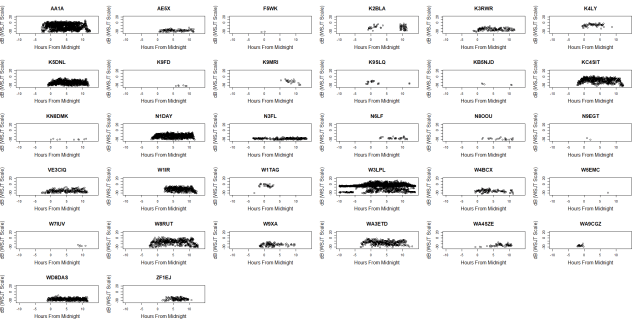
One of the first questions I have had as I am getting started with 630m is, “How well am I doing in terms of my receive system”?

Fortunately, there is a great tool available to all of us for testing our receive systems. That tool is WSPRNET, and we can use it to compare our receive systems with those of anyone else who is uploading their WSPR spots to WSPRNet!

In addition to showing you a map of WSPR spots, WSPRNet will allow you to see a list containing the details of all of the spots uploaded over the past 24 hours (or even as long ago as two weeks) by any station participating. To see these details go to this page and complete it so that is looks something like what is below, and then click “Update”:

Note that I used “W3SZ” as the reporting station. This means that the server will return all of the spots that I heard and uploaded. If I wanted to see what Bill, AA2UK heard, I would enter “AA2UK” into the “reporter” box, for example.

Doing this will give you a screen similar to what is below. I am displaying only a small portion of the spots displayed. The web page will let you display up to 1000 spots, so if it was a busy night you may not get all of the spots from a superstation. I generally leave the count set to 1000 so that I get the data on as many spots as possible, in order to optimize the statistics:

I am certainly NOT a superstation, but you can see that the web page maxed out at displaying 999 of my MF spots for the previous 24 hours and didn’t show the MF spots that I uploaded that were in excess of that.

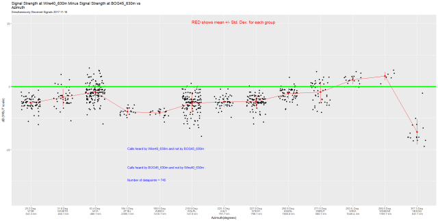
So what can you do with this information? Well, here is a graph that I made using AA2UK’s and my WSPRNet spots from October 30:

The graph shows the DIFFERENCE in signal strength of signals that were SIMULTANEOUSLY received at W3SZ and AA2UK. I calculated the difference as (the signal strength at my station) MINUS (the signal strength at Bill’s station). So if my station receives a signal better than Bill’s station does, then this number will be positive. If Bill’s station receives the signal better, then the number will be negative. You can see from the graph that at azimuths relative to my station of 3, 203, 228, 261, and 290 degrees Bill and I received signals equally well. At 25 degrees I was down by 10 dB, and at 63 degrees I was down by 5 dB.

You can compare this with the graph for simultaneous signals that produced from the data for October 31, shown below:

There are fewer data points, because Bill was chasing DX using other modes, so the data is less statistically robust. Still, while we only heard 7 stations simultaneously the first night, this night we heard 9 stations simultaneously. We copied AA1A at 63 degrees/413 km and K5DNL at 261 degrees/2023 km from my location equally well, Bill copied K2BLA at 203 degrees/1350 km and VE3CIQ at 357 degrees/591km better, and I had possibly better reception for W3LPL, KC4SIT, N1DAY, W9XA, and WD8DAS, whose azimuths and distances from me are shown along the bottom axis of the graph. The data for the second day is statistically weaker due to the smaller dataset, and given the error bars, I would say that overall it looks as though Bill and I are closely matched in terms of our receive capability. So we are doing well, right?

Well, NO!!! Look at the graph below, comparing my reception overnight with that of Mike, WA3TTS:

Mike and I received 12 stations simultaneously, with a total of 683 simultaneous decodes uploaded to WSPRNet. We are about even in terms of our reception of AA1A and W3LPL. But I am 5 dB down for K9FD at 281.3 degrees and 7439 km (he is in Hawaii), and roughly 10 dB down for AE5X, N8OOU, and VE3CIQ. I am roughly 15 dB down for ZF1EJ, KC4SIT, N1DAY, and WD8DAS. I am roughly 20 dB down for K2BLA and K5DNL. Mike is located near Pittsburgh, 347 km from me in EN90xn. So distance does NOT explain my signal deficit for most of the stations noted.

Here is how Mike’s and my signals compared using cumulative data from 10-30 through 11-2. We received 16 stations simultaneously,and the total number of data points was 1254. Mike heard 7 stations that I did not, including some Europeans. I heard only 1 station that he did not:

Mike also outperformed Bill on receive, as is seen on the graph below. Here the results are WA3TTS minus AA2UK, so a positive number means that WA3TTS’s receive performance is superior,and a negative number means that AA2UK Bill’s receive performance is superior. WA3TTS is better by approximately 20 dB for WD8DAS and K2BLA’s signals, and by about 15 dB for N1DAY and K5DNL. There are no stations where Bill outperforms Mike.

Mike is an experienced Lowfer, and he has paid great attention to his receive system and to MINIMIZING noise. Mike gave me these suggestions in one of his extremely valuable emails:

Separate grounding for receive, isolation transformer at receiver antenna input, and a battery for antenna preamp are pretty much essential for serious MF/LF performance. A single BN73202 W8JI beverage transformer should only be a dB or so down in performance at 475kHz, that BN73-6802 “double length” ferrite core about optimal for 630m band for antenna and isolation transformer applications.

You need enough magnetizing force with the toriod material to be efficient at LF/MF, so generally the 73, 77, and 75 materials are used for low-Q broadband efficiency and 61 material reserved for high Q filter applications

Mike also gave me some great references on managing receive noise in general, including for example this web page from W3EEE on reducing EMI noise on receive antennas and this web page describing using an optical link to isolate the antenna from EMI brought from the mains along the feedline from the shack.

Mike also pointed out that for some, overload from AM Broadcast Band transmitters can be a show stopper, and he gave me a link to a schematic for the W1VD Hi-Q preselector.

After seeing how relatively bad my receive performance is by way of the graphs I generated and shared with you above, I am very motivated to start undertaking some of Mike’s suggestions on how to improve my receive sensitivity.

If you are interested in producing similar graphs for yourself once you are starting out on 630m, continue reading below. If you are not, then stop reading here! There be dragons below!!

To do this yourself you need to be computer savvy. IF you are thinking about doing this, then read all of what is below before giving it a try. If you don’t understand any of what is below, turn back now.

There is more detail below than you need to set things up. So I put text that discusses things that you actually need to do to get this going in bold, in order to make it easier to find these “must do” items.

1. Turn on the “Upload spots” function in your WSJT-type software. If you are using WSTJX, then make sure the “Upload spots” function is checked as is shown below:

2. After you’ve acquired a session’s worth of spots, go to this page and complete it as outlined above, setting the maximum number of downloaded spots to 999, entering your call in the REPORTER box, and then clicking on “Update”.

3. Then, once the spots have appeared, left click and scroll and once you have selected all of the spots, right click and click “Copy” to save them to the clipboard.

4. Then open your favorite text editor that will allow you to save a simple “.txt” file, open an empty document, and right click on the document and then click “Paste”. Then save the document as “Whatever.txt”.

5. Now repeat steps 2 through 4 above, but this time in the “REPORTER” box place the receive station with which you want to compare yourself.

6. For this example below, rather than comparing myself with another station, I will compare WA3TTS (the primary station) with K3RWR. This means that receive signal strength differences will be expressed as (Signal Strength at WA3TTS) minus (Signal Strength at K3RWR), and azimuth and distances to the received stations will be given the values for WA3TTS.

7. Download and install R from here. You want one of the precompiled binary versions, NOT the source.

8. Download and install the free version of R Studio Desktop from here.

9. Start R Studio and go to the “Packages” window in the lower right hand corner and install, if they are not already listed there as being installed:

ggplot2
foreach
sqldf
dplyr

10. Now click on “File >> New File >> R Script to open a new empty script file and copy and paste the code from this file into it:

11. Save the code by clicking “File >> Save” while the source code window has focus.

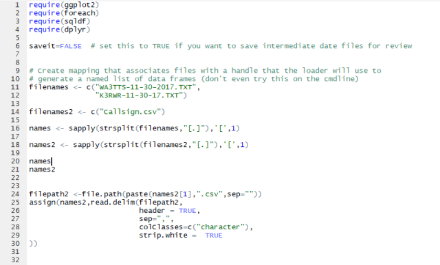
12. The beginning of the script will look like the image below.

13. The first four lines:

require(ggplot)
require(foreach)
require(sqldf)
require(dplyr)

load libraries that are needed to process and display the data. You can find out more about each of these if you want by Googling, “R ggplot” or “R foreach”, etc.

14. The next line,

saveit=FALSE

sets a flag that causes the script to delete many of the intermediate files it creates just before it finishes. Setting saveit to TRUE may help with debugging if things are not working as expected.

15. The next two lines, 11-12,

filenames <- c("WA3TTS-11-30-2017.TXT", "K3RWR-11-30-17.TXT")

define the two WSPRNET data files that you created as above, and want to analyze with this script. For this example they are “WA3TTS-11-30-2017.TXT” and “K3RWR-11-30-17.TXT”. These files NEED TO BE PLACED IN THE SAME DIRECTORY AS YOUR R SCRIPT FILE.

Changing these two file names to the names that you used when you created the two WSPRNet data files above are the ONLY changes that you should need to make to the script code!

16. The next line,

filenames2 <- c("Callsign.csv")

refers to a csv file that you need to create if you want to create and display a list of “new” stations heard.

17. You need to create this csv file named Callsign.csv and put it in the same directory that has your R script file. This file needs to have 1 column, named Callsign. You need to create in this file a row for each station that you have previously spotted, and in that row to supply in the appropriate column the callsign of that station. This script will import this spreadsheet into R, and once imported the spreadsheet should look like this:

18. Lines 16-21 just separate out (and print in the console, for debugging purposes) the main part of the file names to be compared, dropping the “.TXT” or whatever the file extensions are:

When the script is run, this portion of the script will produce the console printout:

Of course, the actual file names listed under “names” will be the names that you gave your WSPRNet files when you created them above.

19. Lines 24-30 import the Callsign.csv file into R Studio:

20. Lines 33-44 import the two WSPRNet files to be compared into R Studio:

21. The remaining code sets up the graphs and then displays them. If you want to learn more about the details of that code, Google is your friend. But I have written the code to be “generic”, and the only code details that you need to know to do all of this at your location are explained above.

22. Create a subdirectory named “Images” in the directory where you have saved the R script file. This is where your graph files will be placed.

23. Now you should be ready to create your first graphs. Left-click and scroll to select the code and then run it by clicking Control-Enter or clicking the “Run” icon at the upper right corner of the code window. If there are no errors, then RStudio will display two graphs in the lower right quadrant Plot window, and write the plots to “../Images/filename_1_filename_2_Vs_Azimuth.PNG” and “../Images/filename_1_filename_2_Vs_Call.PNG”, where filename_1 and filename_2 are the names of the two files being compared. If you want to put the graph files elsewhere, then you need to change the code appropriately. Or you can just click on “Export” above the displayed graphs and then select the directory and file names that you want to use to store the graphs.

24. Look in the Console window at bottom left to see what calls were unique to each station.
For this set of data, I see:

The graphs produced by this data and script look like this:

25. If things don’t look as they should, then look in the console for error statements. Don’t worry about warnings.

73 and Good Luck!

Roger
W3SZ

There was not much new overnight on 630m. I had 250 simultaneous decodes on both antennas bringing the number of simultaneous decodes since I put up the new antenna on Saturday 10/28 to 604.

There were no new stations copied.

There were 8 stations simultaneously copied on both antennas, so I could calculate the difference in signal strength between the two antennas on those stations’ signals simultaneously received on the two antennas. I wanted to gather this data to see if it provided a possible explanation for why the higher, slightly longer inverted L is the poorer performer.

The data is shown below. The y axis is the difference in signal strength for WSJT signals simultaneously received by the two antennas. It is shown as superior 125-degree-axis signal strength minus inferior 35-degree-axis signal strength. The x axis is the azimuth from W3SZ to each station providing a simultaneously received signal. This is of course a discrete and not a continuous variable, which is why the x axis is scaled as it is.

Note that the horizontal axis, although it shows azimuth values in an ascending monotonic fashion, is not linear or smoothly distributed. Neverthless, it looks like there is greater superiority (by about 5 dB) of the 125-degree-axis antenna over the 35-degree-axis antenna at an azimuth of roughly 25 to 65 degrees as compared to other azimuths. Because there are no datapoints between roughly 65 degrees and roughly 205 degrees, the exact azimuth of this “peak” cannot be determined. However, there does not appear to be ANY direction in which the 125-degree-axis antenna is not superior to the 35-degree-axis antenna.

Why is the 125-degree-axis antenna superior in all directions assessed even though it is shorter and lower?

Both antennas are imperfect, with the feedline not running perfectly vertically from the ground to the horizontal element in either case. In this respect, the inferior 35-degree-axis antenna is more nearly perfect. Also, the 35-degree-axis antenna is very close to being perfectly horizontal, while the 125-degree-axis antenna has a slight upward tilt looking down its axis away from the feedpoint. The 125-degree-axis antenna also has a slightly longer feedline running along the ground to the LNA. The 35-degree-axis antenna’s feedline comes right down from the feedpoint, enters the small antenna control hut, and attaches to the LNA without ever reaching the ground. Both LNAs are grounded to a ground rod right beneath them.

Inverted L antennas are complicated beasts, with their properties very much dependent on their length relative to the wavelength at which they are used, and on the length of the feedline (vertical segment) vs the length of the upper horizontal segment. They are actually fairly omnidirectional when properly dimensioned, and several sources have indicated that they are the best “simple” antenna that one can erect.

There is an excellent review of Inverted L antennas by none other than L.B. Cebik here. Then click on “Inverted-L – Cebik.pdf. The website on which this file is located is protected and you can’t get to the file directly, but going to the directory and then clicking on the file name as just suggested will get you the pdf file.

I suspect that it is a combination of site-specific and installation-specific factors that cause the difference in antenna performance that I am seeing.

I do have star-configuration grounds around each tower, and a large conductor runs from the tower farthest from my shack to the shack, running relatively parallel to the inferior 35-degree-axis antenna and roughly perpendicular to the 125-degree-axis antenna. Perhaps that is playing a role. Or perhaps the fact that the inferior antenna is attached (via insulating cord) to relatively tall towers that extend far above it at each end of its length degrades its performance.

I will have a chance to gather more data and will report back any further useful information that I get in this regard.

73,

Roger
W3SZ

I am currently exploring the 630m band primarily by monitoring WSPR broadcasts, in order to get a sense of what propagation is like, and what my receive capabilities are.

I have two openHPSDR Hermes transceivers at Hilltop, each one hooked up to an inverted L antenna fed with hookup wire which is connected to its own AMRAD Active Antenna LNA.

One of antennas has its axis (looking away from the feedpoint) at 35 degrees azimuth, and the other has its axis looking at 125 degrees. The 35-degree-axis antenna is slightly less than 50 feet long. The other is about 40 feet long. The axes for both are shown in the Google Maps satellite views below:

Although the 35-degree-axis antenna is higher, at 15 feet vs 8 feet for the 125-degree-axis antenna, the 125-degree-axis antenna performs much better. Perhaps this is because the 35-degree-axis antenna is adversely affected by the towers at each end of its course.

You can see this on the graphs below, one for each callsign detected last night, showing the signal strength in WSJT dB units vs time as HH:mm. The 125-degree-axis antenna is pink in each graph, and the 35-degree-axis antenna is blue. There are 5 stations for which ONLY the 125-degree-axis antenna garnered any decodes.

Many stations don’t leave their equipment on during the day, and some of the individual station “start” and “stop” times may reflect this, rather than propagation. Also, for the same reason, one can’t assess night vs day from these graphs, even though I continued to record data throughout the day. Here are the graphs, in ascending azimuth order:

Here is a plot of average signal levels over time starting at 0000 UTC and continuing until there were no more stations heard. The signal strengths do appear to drop off around sunrise:

That’s all for today!

73,
Roger
W3SZ

To see my website, please go to:

http://www.nitehawk.com/w3sz